Autocad_Volumetrics

Introduction

This tutorial describes how to use Key TERRA-FIRMA to calculate volumes from ground models (.KGM files) and how to calculate cut and fill volumes between ground models. It assumes that you have completed the "Ground Modelling" tutorial or that you already have a good understanding of TERRA-FIRMA's ground modelling features. The tutorial goes on to explore the various ways to graphically present cut and fill data using TERRA-FIRMA's contouring and elevation analysis tools.

Those of you who need only a quick step-by-step guide or a refresher can go straight to the FastTrack section of the tutorial.

Cut & Fill

"Cut and fill" or "Volumetrics" is the calculation or analysis of landform volumes. It may be desirable to change the existing landform of a site for a number of reasons. For example, a sloping site will require platforms for buildings and car parks, visual screening bunds may be required at the site boundary or a lake may be created. Landform modification is a very common site design requirement and one in which landscape architects are often involved.

The movement of large quantities of material to and from a site can be extremely costly. In order to minimise this cost it is often desirable to design a landform which uses only material found on a particular site. It is important, therefore, to know what volume of material you are starting with and what volume of material the designed landform will require. Ideally the two volumes will be the same. In such a case, no imported material is required, neither does any material need to be exported, thus minimising cost. This ideal situation occurs when the landform designer has balanced the cut and fill.

A "Cut" volume is defined as the volume of material which is excavated below existing site levels. "Fill" volume is the volume of material which is mounded above existing site levels. Cut and fill volumes are expressed in metres cubed (m³).

Download Sample Data

If you have no contour data to work with you may like to download a sample file so that you can follow the live tutorial. Click on the icon below to download the AutoCAD drawing file gm-base.dwg. Even if you have your own contours you may like to use this file for the purposes of the tutorial before you start work with your own data. There are two download options, you can either download the native AutoCAD drawing file or you can download the smaller compressed version. The Zip file can be uncompressed with a utility such as WinZip.

 gm-base.dwg (183KB) - AutoCAD R14 Drawing File

 gm-base.zip (73KB) - Zipped Drawing File

The drawing file is approximately 2km x 2km square and contains two sets of contours on different layers (see illustrations below). The contours are at 5m intervals in the range 175m to 395m with index contours drawn at 25m intervals. The drawing contains three sets of contour layers:

1. EXIST_CONT_05M and EXIST_CONT_25M contain the existing contours before modification.
2. QUARRY_CONT_05M and QUARRY_CONT_25M contain the design contours for the quarry.
3. COMMON_CONT_05M and COMMON_CONT_25M contain those which are common to both.

In addition to the contour information, the drawing includes a number of spot heights that are used to define the flat bottom of the quarry. The spot heights are block objects called "LEVEL".

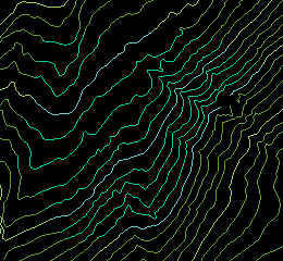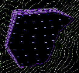Existing and common contours, showing the landform before modification.	Design and common contours and spot heights, showing the proposed landform.

The two contour sets can be viewed as in the illustrations above by selectively turning off the "quarry" layers and the "exist" layers respectively. See the "Object Properties" tutorial to find out about turning layers off and on.

Creating the Ground Models

The first stage in doing a cut and fill analysis involves creating the ground models which will be used. Follow the steps below to create two ground models from the sample data or create two of your own ground models. In order to follow the tutorial, you will need to download the GM-BASE AutoCAD file and create two ground models.

1. Download the GM-BASE drawing and save it to an appropriate folder.
2. Start Key TERRA-FIRMA by double-clicking on the program icon and open the GM-BASE drawing.
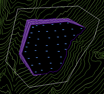
3. Create a new layer called "ACTIVE-PASSIVE", make it the current layer and draw a closed Polyline around the quarry area as shown in the illustration above.
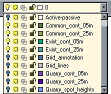4. Using the Object Properties toolbar, turn off all layers except the "Common" and "Exist" layers. Your Layer Control pull-down should look like the one in the illustration below.
5. Create a ground model from the visible contours. This ground model represents the existing landform.
   
   Use the Create Ground Model command,  from the toolbar or KeyT-FCreate Ground Model… from the pull-down. See the relevant section in the "Ground Modelling" tutorial if you are not sure about using this command.
   
   Make sure that you correctly specify all the required layers in the 2D Polyline Layer Definition dialogue box (see illustration). Also, deselect the "Breakline Recognition" option, it is not required for this model and model creation will be much faster without it. Call the new ground model file "exist".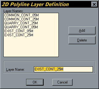
6. Using the Object Properties toolbar again, turn off the "exist" layers and turn on the three "quarry" layers.
7. Create a second ground model from the visible contours and spot heights. This ground model represents the designed landform.
   
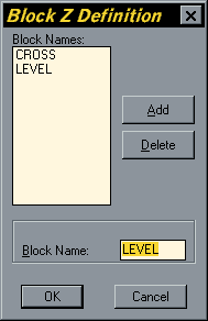   This ground model will be created using both contours and spot heights so you must select the "Blocks (Z Value)" option and specify the the block name "LEVEL". Type "level" in the "Block Name" text box and then click the "Add" button. The block name "LEVEL" will be added to the "Block Names" list. See the illustration on the right.
   
   Call this ground model "quarry".
   
   You should now have two ground models which could be used to run a cut and fill analysis as they stand. However, a large proportion of the two ground models are the same and in these areas the cut and fill will balance and cancel each other out. The only area of change is where the quarry will be excavated. It would be most efficient, therefore, to define the quarry area as an active zone within each ground model. This will have the advantage of speeding the whole calculation process up.
8. Turn on the "ACTIVE-PASSIVE" layer and define active/passive zones for both ground models using the closed Polyline you drew earlier as the boundary. You can access this command by clicking  from the Ground Modelling toolbar or KeyT-FActive/Passive zonesDefine from Polyline(s)… from the pull-down. If you need more information about active/passive zones, see the relevant section of the "Ground Modelling" tutorial.

You now have all the base material required to complete the cut and fill calculations.

Volume Commands

Key TERRA-FIRMA provides a number of methods for calculating volumes. This tutorial covers the two most useful options:

1. The calculation of volume between one ground model and a horizontal plane using the Model information command
2. The calculation of volume between two ground models using the Prismoidal Volumes command.

Both of these commands use a prismoidal method for calculating volume. This method is generally accepted to be the most useful and accurate for general purpose volumetrics. You may have noticed that TERRA-FIRMA also offers the option to calculate volumes by a sectional method. This type of volume calculation is most appropriate when the calculated volume is linear in planform. It is usually used for volumetrics calculations relating to road and rail schemes.

Model Information

Toolbar
Pull-down	Key T-FModel Modifications and InformationModel information…
Keyboard	none

The Ground Model information command can be used to display all relevant information about a ground model file (.KGM). A ground model must be created before this command is used. The Ground Model Info dialogue box is shown below. As you can see, this command can be used to calculate the volume below any ground model.

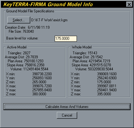
The dialogue box is divided into three sections. The "Ground Model File Specifications" section gives information such as the full path name of the file, the date and time that the file was created and the file size. This section also contains an edit box which allows you to specify the base level for any volume calculation. By default, this value is set to the minimum Z value in the ground model. This ensures that the entire ground model will be used when generating areas and volumes. The sections below show what happens to the calculated volumes when this value is changed. Notice that it is not possible to generate a volume with a base level above the minimum Z value.

The Ground Model Info dialogue box also contains sections entitled "Active Model" and "Whole Model". The Active Model section shows information which relates to that part of the model which has been defined as "Active" using the Active/Passive Zones command. If no active/passive zones have been defined, the whole model is active and the contents of this section will be identical to that in the Whole Model section.

Calculating a Volume

To calculate the volume below any ground model, simply start the Model Information command, select the ground model file, set the base level and click on the "Calculate Areas And Volumes" button. In a few seconds the results will be displayed in the Ground Model Info dialogue box.

In theory you could, in fact, do a cut and fill calculation based on the above method. Simply calculate the volume below any two ground models of the same extent (or with the same active/passive zones defined) and with the same base levels. Subtract the volume of the existing ground model from that of the proposed ground model. A negative result will give you the volume of cut, a positive value will give you the volume of fill. If both cut and fill are perfectly balanced, the result would be zero.

Although this method will give you a satisfactory cut/fill value, it is impossible to tell how the total is arrived at. For example, a gross figure of 10,000m³ fill might be arrived at by cutting 10,000m³ and then filling 20,000m³ or it may simply be arrived at by filling 10,000m³. Obviously the cost implications of the two possibilities are quite different. The Prismoidal Volumes command should be used where you need more information about a cut/fill calculation.

Prismoidal Volumes

Toolbar
Pull-down	Key T-FVolumes and IsopachytesVolumes (Prismoidal)…
Keyboard	none

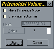The Prismoidal Volumes command is specifically designed for cut and fill calculations. The command works by comparing one ground model with another. In most cases this will be one ground model representing the existing landform and another representing the proposed landform. The latter is usually referred to as the "Design Ground Model".

The first thing you see when starting the Prismoidal Volumes command is the Prismoidal Volumes dialogue box, shown on the right. As you can see, the dialogue box offers a couple of options, namely, to create a difference model and todraw an intersection line. Both of these options are covered later in this tutorial.

A Cut and Fill Calculation

Follow the next section of the tutorial to generate cut and fill statistics from the two ground models you created earlier.

1. Start the Prismoidal Volumes command. Deselect "Create Difference Model" and "Draw intersection line" if they are selected. The dialogue box should look like the one in the illustration above. Click on the "Start" button.
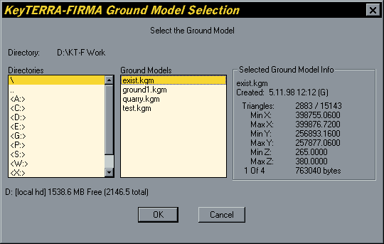
2. When the Ground Model Selection dialogue box appears, select the ground model file (.KGM) which represents the existing landform, often called the "Survey" ground model. If you have been following this tutorial, the file is called exist.kgm, see the illustration above. Having selected the file, click on the "OK" button.
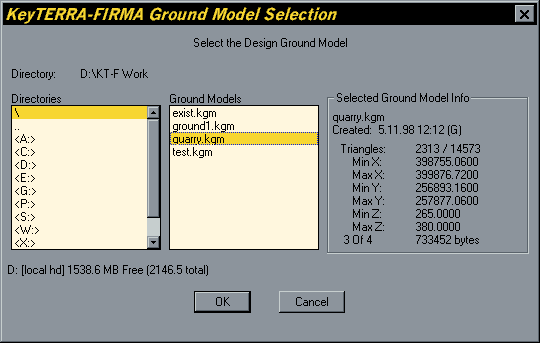
3. The Ground Model Selection dialogue box appears again but this time you are prompted to select the "Design Ground Model". Select the file calledquarry.kgm and click on the "OK" button.The cut and fill calculation will now start. This process will take between just a few second and perhaps a few minutes depending upon the complexity of the two ground models and the speed of your computer. You can get an idea of the speed of the calculation by looking at the progress indicator which appears on the AutoCAD status bar, see the illustration above.
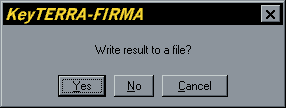
4. When the calculation is complete, TERRA-FIRMA asks whether you would like to write the results of the calculation to a file. This is usually a good idea because otherwise you will have to write down the figures from the AutoCAD command line. Click the "Yes" button to write the results to a file.
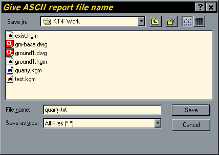
5. When the "Give ASCII report file name" dialogue box appears, enter a suitable name in the "File name" edit box. The report file which will be created is a plain text file, otherwise known as ASCII. Such a file can easily be viewed using Notepad. In order to link the report file with Notepad, you need to give the file a .TXT extension. All files with a .TXT extension will automatically be opened using Notepad when they are double clicked. To ensure that the report file is saved as the correct file type, enter a name such as "quarry.txt" in the File name edit box. Click on the "Save" button to save the report file.Once the report file has been created, the cut and fill results are also written to the command line so that you can immediately see the results of the calculation, see the illustration above.

If you look closely at the command line illustration above you will notice that although the quarry ground model was created entirely by cutting the existing landform, there is small amount of fill recorded in the results. This is largely caused by small differences between the two ground models at the boundary where the two models diverge. If you look at the actual figures involved, the figure given for fill represents about 0.016% of the balance. This is well within the acceptable tolerance for such a calculation.

Creating a Difference Model

The Make Difference Model option of the Prismoidal Volumes command enables you to create a ground model which represents the difference between the existing and design models. This is done by subtracting one model from the other. The Z values of the resulting ground model represent the amount of cut or fill. Negative Z values represent cut and positive values represent fill. Where the two ground models are the same the Z values will be zero. When you have created a difference model, you can contour it to produce contours of cut depth and fill height known as isopachytes.Contours can be generated using theContours command. The difference model could also be used to create colour coded areas on a plan to represent areas of cut and fill. This could be done using the Elevation Analysis command.

To create a difference model during the cut and fill calculation process, simply check the box against the "Make Difference Model" option in the Prismoidal Volumes dialogue box before clicking on the "Start" button. After the report file has been created (assuming you want one), TERRA-FIRMA displays the Create Differential Model dialogue box, illustrated below.

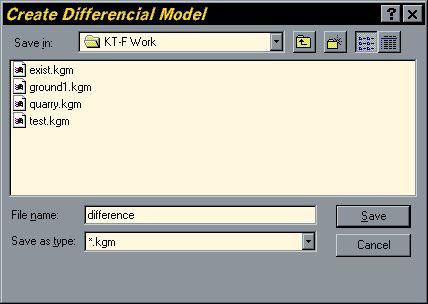
Simply enter a filename such as "difference" in the "File name" edit box and click the "Save" button. Note that you do not need to add a .KGM file extension as this will automatically be done for you.

Drawing an Intersection Line

The Prismoidal Volumes command also enables you to draw an intersection line which marks the intersection of the two ground models (assuming they do intersect). Effectively this line marks the boundary between areas of cut and areas of fill. This line also represents the zero contour (isopachyte) on a difference model.

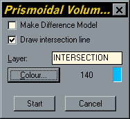To draw an intersection line during the cut and fill calculation process, simply check the box against the "Draw intersection line" option in the Prismoidal Volumes dialogue box before clicking the "Start" button. You will notice that when this option is checked, the "Layer" and "Colour" options become available (previously they were greyed out), see the illustration on the right. Use these options to define a layer name and layer colour for the intersection line. A new layer will automatically be created with the specified name and colour settings. The intersection line will be drawn during the calculation process.

Contouring

Toolbar
Pull-down	Key T-FContours…
Keyboard	none

The Contour command can be used to generate contours from any TERRA-FIRMA ground model. The Draw Contours dialogue box is shown below. As you can see, there are a number of options which have to be set in order to generate the particular contours which may be needed in any particular circumstance.

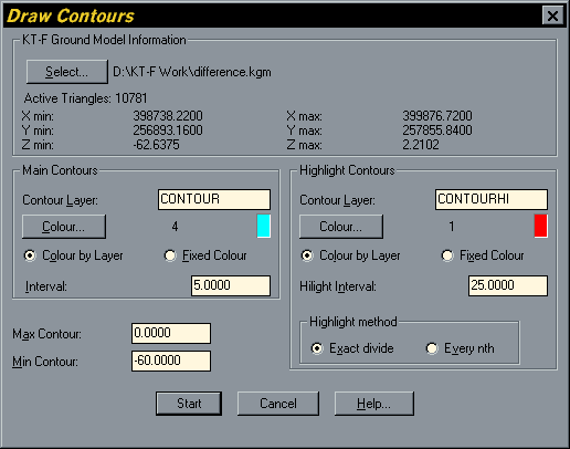
The dialogue box is divided into a number of sections. Use the "Select…" button in the "KT-F Ground Model Information" section to select the ground model from which contours are to be generated. In many cases the correct ground model will already have been selected automatically.

Use the "Main Contours" section to specify the layer and colour of the contours. Also, most importantly, set the value for the contour interval. By default, the contour interval is set to 1, however this may not be appropriate in every case.

The "Highlight Contours" section of the dialogue box is used to specify the layer, colour and interval for the highlight or index contours. Index contours are commonly used on maps to make the contours easier to read.

Finally, the Max Contour and Min Contour values must be entered. By default, these values are set automatically from the range of Z values in the ground model and rounded to the nearest metre. However, if you want a contour interval of 5 metres, you will need to make sure that the Min Contour value is rounded to the nearest 5. For example, if the default Min Contour value is -63 and you want to generate 5m contours, you will need to change this value to -60.

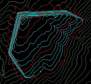
The illustration above shows the result of contouring the difference model created earlier in this tutorial. A 5m contour interval has been used with index contours at 25m intervals.

Follow the steps below to generate contours for the difference model.

1. Start the Contour command
2. Use the "Select…" button to select the difference ground model file.
3. Set the contour interval to 5 in the "Main Contour" section of the dialogue box.
4. Set the Highlight Interval to 25.
5. Set the Max Contour value to 0 (zero), and the Min Contour value to -60. The settings in the dialogue box should now look the same as the ones in the dialogue box illustration above.
6. Click on the "Start" button and the contours will be drawn. Contouring usually takes just a few seconds. When contouring is complete, your drawing should look similar to the illustration above.

In this particular example the contours represent the depth of cut. Since there are no contours greater than zero, no fill is indicated.

If you are not necessarily interested in showing the depth of cut or fill but simply wish to indicate whether an area is in cut or fill, you could use the Elevation Analysis command to create solid colour bands to show this. See the section below for details.

Elevation Analysis

Toolbar
Pull-down	Key T-FSite AnalysisElevation…
Keyboard	none

The Elevation Analysis command can be used to calculate the percentage area coverage of different elevation bands within any TERRA-FIRMA ground model. It can also be used to create a three dimensional triangular model of the terrain surface with triangles colour coded by layer for each elevation band specified. These triangles can either be 3D Faces or they can be Solids.

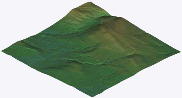
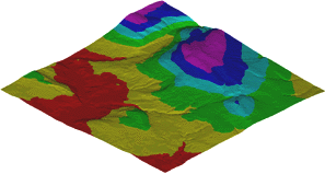The image on the right was produced by rendering an elevation analysis created from 3D Faces. Six elevation bands were used and the band colours are the defaults set by TERRA-FIRMA. As you can see, this produces a clear visual analysis of ground model heights which works well in both 3D views and in plan. If you are working mainly in plan, it may be more efficient to create the triangles using Solids since they do not need to be rendered to give a solid colour effect. The image below shows the same analysis but this time the elevation band colours have been changed to make the distinction between bands more subtle and to more closely mimic real terrain colours. The highest band uses AutoCAD colour number 53, the others are coloured 63, 73, 83, 93 and 103 for the lowest. The change in colour was achieved simply by changing the layer colour of the various elevation bands with the Layers command,  from the Object Properties toolbar. The way AutoCAD colours display may vary depending upon your graphics card and monitor so it's always best to experiment with colours to get the best effect.

In the example above, the elevation bands were set so that each colour represents a 50m elevation difference. The range in elevations within the model is approximately 100m to 400m. The red band represents elevations between 100m and 150m, the yellow band represents elevations between 150m and 200m and so on. You can use the Model Information command,  to find the elevation range within any ground model. The elevation range is expressed as Z min, the lowest and Z max, the highest. It's a good idea to do this before starting the Elevation Analysis command so that you can work out the number of bands you need and the range within each band.

The methodology outlined above holds good for most cases where an elevation analysis of a ground model is required. For some specific cases, however, you may need to create an elevation band set where the elevation difference is not the same for all bands. This is true for the presentation of cut and fill areas on a difference model. Follow the sequence below to create a map of cut and fill areas using the difference model created earlier in this tutorial.

1. Start the Elevation Analysis command,  from the 3D Site Analysis toolbar or Key T-FSite AnalysisElevation… from the pull-down menu.
2. When the Ground Model Selection dialogue box appears, select the ground model file (difference.kgm) from the Ground Models list. If you did not previously check the elevation range in the model, you can do so now by looking at the Max and Min Z values shown in the "Selected Ground Model Info" section of the dialogue box. Click on the "OK" button.
3. When the Regions of different Elevations dialogue box appears, click on the "Add…" button.
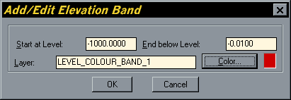
4. Clicking the "Add…" button brings up the Add/Edit Elevation Band dialogue box, shown above. This dialogue box is used to specify the elevation range within each band and the colour that any 3D Faces or Solids that may be created.
   
   In order to correctly illustrate areas of cut and fill, we will need to define 3 elevation bands, one representing cut, one for fill and one where there is no change. The elevation range for cut will be from -1000 up to -0.01 , the range for "no change" will be from -0.01 to 0.01 and the range for fill will be from 0.01 to 1000. It does not matter that the maximum value in the fill band and the minimum value in the cut band exceed the actual ground model values. Part of the reason for going up to 1000 in each case is so that we can save this band set for use on future cut and fill analyses and there will not be many occasions (if any) where these values are exceeded. The figures for "no change" are notional, but reasonable in the context of such ground models. Effectively what we are saying is that any change between minus one centimetre and plus one centimetre is considered to be "no change".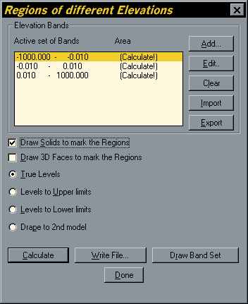
   
   Enter the value -1000 in the "Start at Level" edit box and the value -0.01 in the "End Below Level" edit box. A new layer will automatically be created for each new elevation band. Use the Layer edit box if you wish to change the default name for this layer and click on the "Color…" button to change the default colour. Rremember, you can always change the layer colours at a later time since colours are assignedByLayer. See the Layers section of the Object Properties tutorial to find out how to change layer names and colours. When you have finished defining the elevation band, click on the "OK" button. You will be returned to the Regions of Different elevations dialogue box and the first band will appear in the "Active set of Bands" list.
   
   Click on the "Add…" button a second time and define the second band (-0.01 to 0.01). Complete the band definitions by clicking "Add…" a third time and enter the values 0.01 and 1000. The Regions of different Elevations dialogue box should now look similar to the one in the illustration above. If you have made a mistake, you can always correct it by selecting the incorrect band from the list and clicking on the "Edit…" button.
5. The process of band set definition can be quite time consuming, especially where you are dealing with complex band sets. It is therefore often a good idea to save the band set definitions to a file for future use.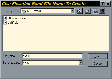Do do this, click on the "Export" button. When the dialogue box appears, enter a file name such as "cut-fill" in the "File name" edit box and click on the "Save" button. Notice that band set definition files have a ".ELE" file extension. These files are usually known as elevation files. To use this file again in the future, simply click on the "Import" button in the Regions of different Elevations dialogue box and select the appropriate elevation file from the list.
6. Now that the band set definition is complete, you can continue with the analysis process. The next decision you need to make is whether you want to create Solids, 3D Faces, both Solids and 3D Faces or neither of these. You can check or uncheck the boxes next to each option as appropriate. For the purposes of this cut and fill analysis it is probably most appropriate to create Solids only.
7. Finally, make sure that the "True Levels" option is selected and click on the "Calculate" button.
   
   The first thing you should see is the percentage area figures appear against each elevation band in the "Active set of Bands" list. Once this is complete, the Solids will be drawn. Your drawing should now look something like the one in the illustration below.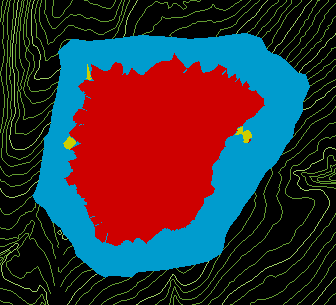
   
   The area of cut is shown in red, the areas of fill in gold and the area of no change in blue. In theory, of course we should see no areas of fill because the area of the quarry has been excavated and no material deposited. However, as mentioned above, small changes at the junction between the two ground models have resulted in a small area of fill representing about half a percent of the analysis area and about 0.016 percent of the volume. This is acceptable in the context of such an analysis.
8. When the calculation process is complete, you are left with another couple of options before finishing the Elevation Analysis command.
   
   The "Write File…" button can be used to write the elevation statistics to an ASCII text file for future reference. The data written to file includes the plan areas of each elevation band in m² as well as the percentage.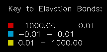
   
   The "Draw Band Set" button can be used to draw a legend for the analysis. The illustration on the right shows the result of using the "Draw Band Set" button for the above analysis. You will be prompted for a text scaling factor. This will vary depending upon drawing size and plot scale so you may have to use some trial and error to get it right. A value of 20000 was used for this example. Before you draw a band set legend you must make sure that the units angle direction is set to North and Clockwise. Use the Units command to set this FormatUnits… from the pull-down menu.
9. Click on the "Done" button to end the Elevation Analysis command.

If you have followed this tutorial from the beginning you should now have a range of tools at your disposal to both make cut and fill calculations and to present the data statistically and graphically.

Volumetrics - FastTrack

1. Create a ground model with existing survey data using the "Create Ground Model" command.  from the Ground Modelling toolbar or KeyT-FCreate Ground Model… from the pull-down. Turn off "Breakline Recognition" for speedier processing.
2. Create a ground model from proposed or "design" data as above.
3. Apply active/passive zones to the two ground models as required.  from the Ground Modelling toolbar or KeyT-FActive/Passive zonesDefine from Polyline(s)… from the pull-down. Make sure that you apply exactly the same active/passive zones to both ground models so that the program is comparing "like with like" when the cut and fill calculation is made. If the two active/passive zones are not the same, the program will only consider the common area when calculating cut and fill.
4. Start the Prismoidal Volumes command,  from the Ground Modelling toolbar or select KeyT-FVolumes and IsopachytesVolumes (Prismoidal)… from the pull-down menu. Check any options you require such as "Draw intersection line" and "Make Difference Model" and then click on the "Start" button.
5. Select the "Survey" ground model from the Ground Model Selection dialogue box and click the "OK" button.
6. Select the "Design" ground model from the dialogue box and click "OK".
7. The cut and fill calculation commences. Calculation progress is shown on the status bar and the calculation results are written to the command line.
8. Choose "Yes" to write the results to a file or "No" to end the command.
9. Check the results to make sure they are what you expected. If necessary, repeat the process until you are quite sure everything is right.

Tips & Tricks

• Always double check your contours for errors before creating a ground model.
• The Prismoidal Volume command will only compare the common area between any two ground models, so it is not necessary that the ground models you are comparing have the same extent. However, if you use the Ground Model Information method, the two ground models must have the same extent so that you are comparing "like with like". If you are unsure about this, always use Active/Passive zones to define the same active zone(s) in each model.
• Whenever you are given the option, save data to file. You never know when it may come in handy and it's easy enough to delete if you find you don't need it.
• Always check the results of a cut and fill analysis to make sure they are reasonable. You should be able to work out a ballpark figure in your head. This will prevent the use of results which are obviously incorrect and will allow you to check your data for problems.
• Always save an "elevation" file when you are defining elevation band sets. The chances are you will run an analysis more than once.